At the “Rencontres R 2018” in Rennes, I proposed a brief introduction to mapping using the recent {sf} package and some other interesting packages. This blog post is an extended version of my presentation allowing me to share the code of the different maps that appeared on it. It’s still a brief introduction.
The original “RR2018” presentation in French is on my github repository
R-code is folded in this blog post, clic on the “CODE” button to unfold it
Mapping in R
All classical operations on spatialized data can be completely performed in :
- Reading and exploration of spatialized / geographic data
- Attributes manipulation (creation, selection)
- Geomatics processing (intersection, joint, surface calculation)
- Map creation (static, interactive)
Packages
library(dplyr)
library(sf)
library(ggplot2)
library(tmap)
library(leaflet)Projections: the ❤️ of the problem
A map is a 2-dimensional representation of all or part of our planet which, sorry to tell you this, is a sphere!
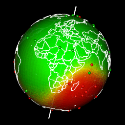
Images of my previous article “spatial interpolation on earth as a 3D sphere”
To create a 2-dimensional map, a projection must be made. The areas you study will be more or less distorted by the projection you chose. One day or another (and it will happen faster than you think!), you will have a problem with a projection. If you don’t know what a projection is, you won’t find the source of your problem! So, if you want to do mapping with R without going through training (such as training at ThinkR for example), you will have to learn and understand what a projection is.
=> Remember your first function sf::st_transform(x, crs) to change coordinate system
Projection of Metropolitan France
I’m not gonna give you a training on projections here. That would be very helpful, but that is not the core of this article. I just present you the map of Metropolitan France that you can download on my github, although these data are originally from the ign website.
Download the data
# extraWD <- "."
if (!file.exists(file.path(extraWD, "departement.zip"))) {
githubURL <- "https://github.com/statnmap/blog_tips/raw/master/2018-07-14-introduction-to-mapping-with-sf-and-co/data/departement.zip"
download.file(githubURL, file.path(extraWD, "departement.zip"))
unzip(file.path(extraWD, "departement.zip"), exdir = extraWD)
}
departements_L93 <- st_read(dsn = extraWD, layer = "DEPARTEMENT",
quiet = TRUE) %>%
st_transform(2154)- 🌍 Geographical coordinates
- In degrees, minutes
- EPSG: 4326
- Used to share data
ggplot(departements_L93) +
aes(fill = CODE_REG) +
scale_fill_viridis_d() +
geom_sf() +
coord_sf(crs = 4326) +
guides(fill = FALSE) +
ggtitle("Coord. géographiques") +
theme(title = element_text(size = 16),
plot.margin = unit(c(0,0.1,0,0.25), "inches"))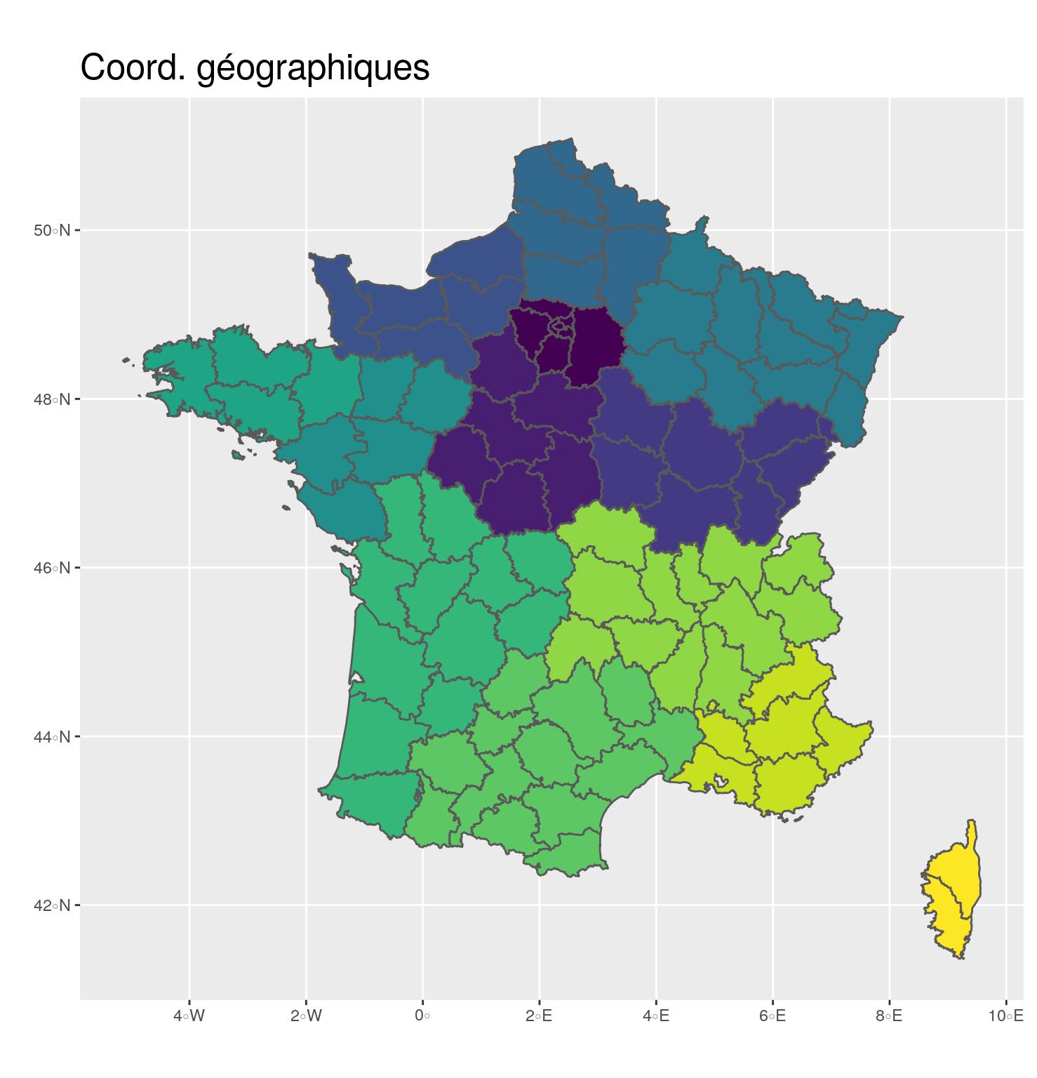
- 🗺 Projection in Lambert 93
- Coordinates in meters
- EPSG: 2154
- A projection to show Metropolitan France on a flat map
g_dept <- ggplot(departements_L93) +
aes(fill = CODE_REG) +
scale_fill_viridis_d() +
geom_sf() +
coord_sf(crs = 2154, datum = sf::st_crs(2154)) +
guides(fill = FALSE) +
ggtitle("Lambert 93") +
theme(title = element_text(size = 16))
g_dept
A GIF to better see the difference
library(magick)
newlogo <- image_scale(image_read(glue("../../static{StaticImgWD}/frwgs84-1.jpeg")), "x1000")
oldlogo <- image_scale(image_read(glue("../../static{StaticImgWD}/frl93-1.jpeg")), "x1000")
image_animate(c(oldlogo, newlogo), fps = 1, loop = 0)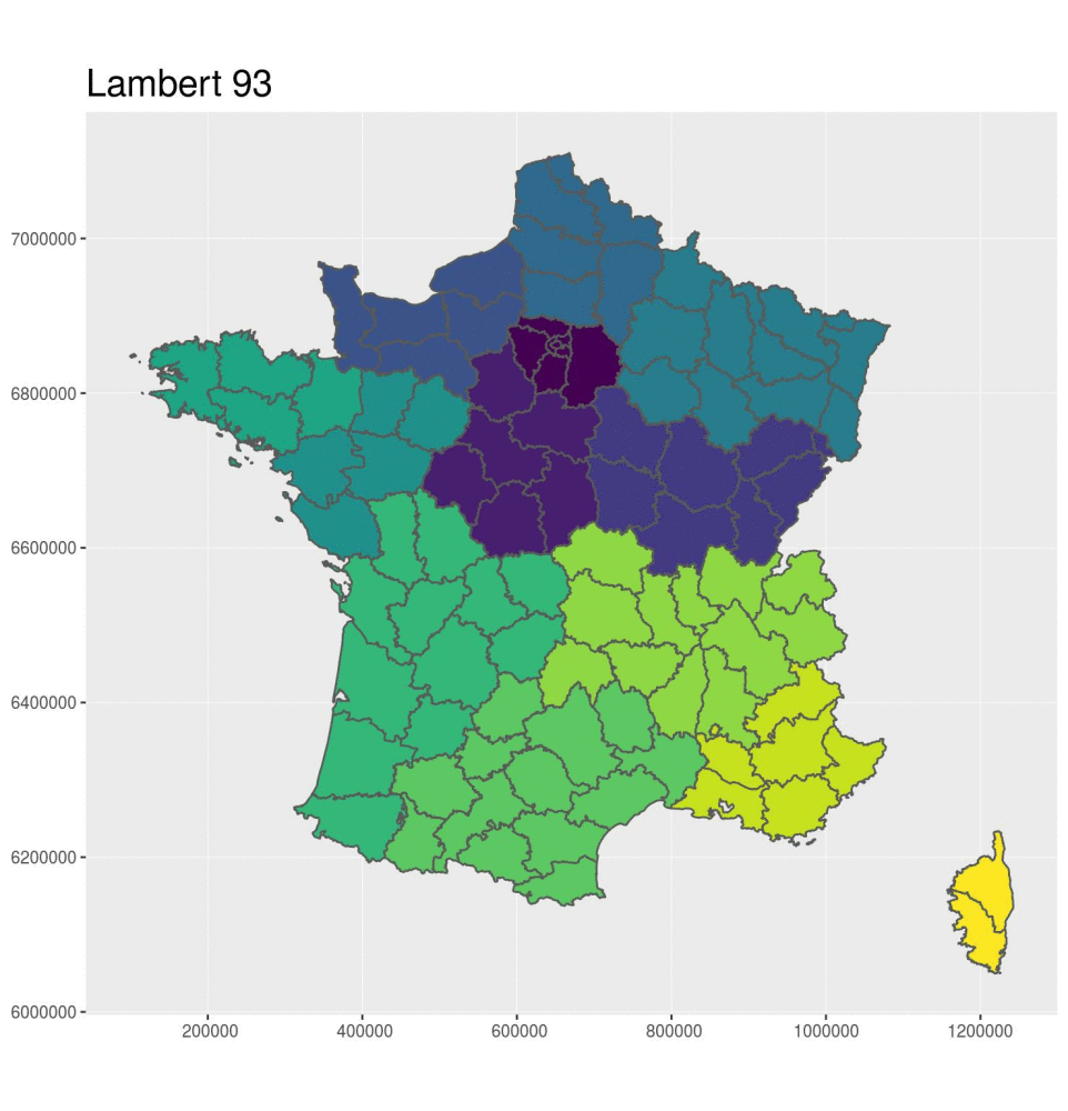
Spatial mapping and analysis with R
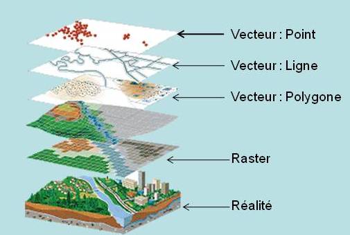
We will focus only on vector data. Raster data manipulation can be realized with the {raster} package, which is very powerful, but this is not the subject of this post.
Vector layer file format
- With {sf} : Read with
st_read.- All formats managed by GDAL (http://www.gdal.org/)
- CSV, Mapinfo, Google Earth, GeoJSON, PostGIS, …
- ESRI™️ shapefile format
- Most commonly shared
- Attention: 4 files minimum (shp, shx, dbf, prj)
- All formats managed by GDAL (http://www.gdal.org/)
With {sf}, the files become classic dataframes.
departements_L93[,2:3]## Simple feature collection with 96 features and 2 fields
## geometry type: MULTIPOLYGON
## dimension: XY
## bbox: xmin: 99217.1 ymin: 6049646 xmax: 1242417 ymax: 7110480
## epsg (SRID): 2154
## proj4string: +proj=lcc +lat_1=49 +lat_2=44 +lat_0=46.5 +lon_0=3 +x_0=700000 +y_0=6600000 +ellps=GRS80 +towgs84=0,0,0,0,0,0,0 +units=m +no_defs
## First 10 features:
## CODE_DEPT NOM_DEPT geometry
## 1 39 JURA MULTIPOLYGON (((886244.2 66...
## 2 42 LOIRE MULTIPOLYGON (((764370.3 65...
## 3 76 SEINE-MARITIME MULTIPOLYGON (((511688.8 69...
## 4 89 YONNE MULTIPOLYGON (((709449.1 67...
## 5 68 HAUT-RHIN MULTIPOLYGON (((992779.1 67...
## 6 28 EURE-ET-LOIR MULTIPOLYGON (((548948.9 68...
## 7 10 AUBE MULTIPOLYGON (((740396.5 68...
## 8 55 MEUSE MULTIPOLYGON (((846578.7 68...
## 9 61 ORNE MULTIPOLYGON (((425026.6 68...
## 10 67 BAS-RHIN MULTIPOLYGON (((998020.8 68...Contrary to {sp} + {rgdal}
str(as(departements_L93[,2:3], "Spatial"), max.level = 2)## Formal class 'SpatialPolygonsDataFrame' [package "sp"] with 5 slots
## ..@ data :'data.frame': 96 obs. of 2 variables:
## ..@ polygons :List of 96
## ..@ plotOrder : int [1:96] 57 12 27 69 76 21 63 18 65 26 ...
## ..@ bbox : num [1:2, 1:2] 99217 6049646 1242417 7110480
## .. ..- attr(*, "dimnames")=List of 2
## ..@ proj4string:Formal class 'CRS' [package "sp"] with 1 slot# str(as(departements_L93[,2:3], "Spatial"), max.level = 3)Manipulate data with {dplyr}
- 🎉 Everything you know of {dplyr} works on {sf} spatial objetcs 🎉
%>%select,mutatefor attributes (= columns)filter,arrangefor spatial features (= rows)
Example of manipulation
Bret_L93 <-
departements_L93 %>%
mutate_at(
vars(NOM_DEPT, NOM_REG),
tolower) %>%
select(CODE_DEPT, NOM_DEPT, NOM_REG) %>%
filter(NOM_REG == "bretagne")
Bret_L93## Simple feature collection with 4 features and 3 fields
## geometry type: MULTIPOLYGON
## dimension: XY
## bbox: xmin: 99217.1 ymin: 6704195 xmax: 400572.3 ymax: 6881964
## epsg (SRID): 2154
## proj4string: +proj=lcc +lat_1=49 +lat_2=44 +lat_0=46.5 +lon_0=3 +x_0=700000 +y_0=6600000 +ellps=GRS80 +towgs84=0,0,0,0,0,0,0 +units=m +no_defs
## CODE_DEPT NOM_DEPT NOM_REG geometry
## 1 35 ille-et-vilaine bretagne MULTIPOLYGON (((330478.6 68...
## 2 22 cotes-d'armor bretagne MULTIPOLYGON (((259840 6876...
## 3 29 finistere bretagne MULTIPOLYGON (((116158.5 67...
## 4 56 morbihan bretagne MULTIPOLYGON (((256230.1 67...ggplot(Bret_L93) +
geom_sf(aes(fill = NOM_DEPT)) +
scale_fill_viridis_d()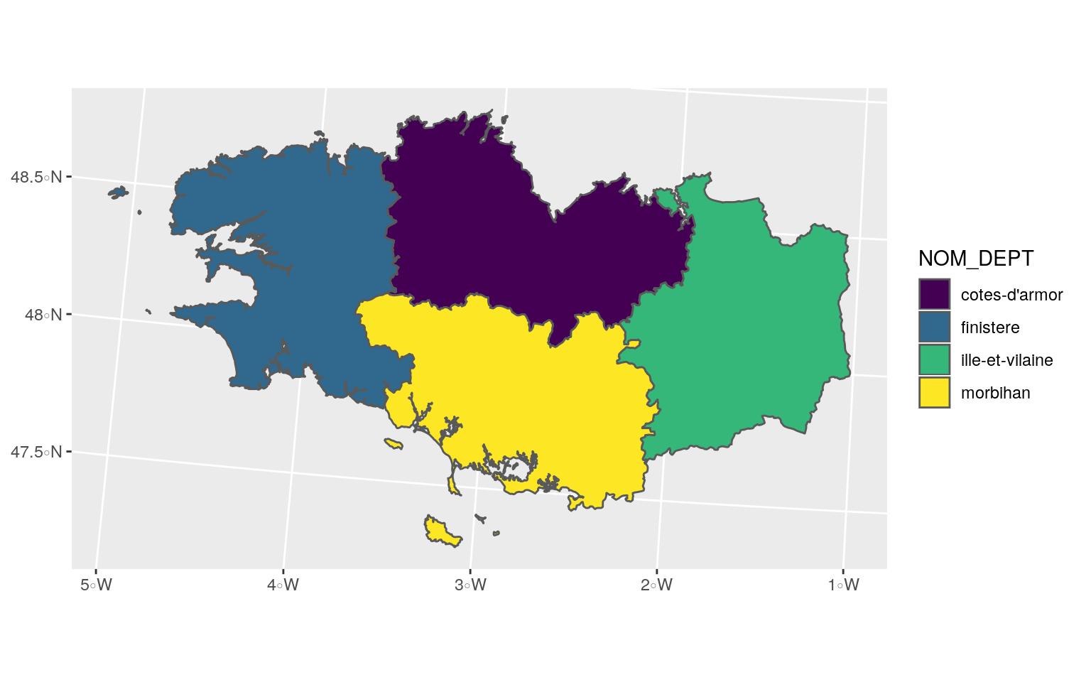
- Merge spatial features with
group_by+summarize
Before
g_dept +
ggtitle("Départements")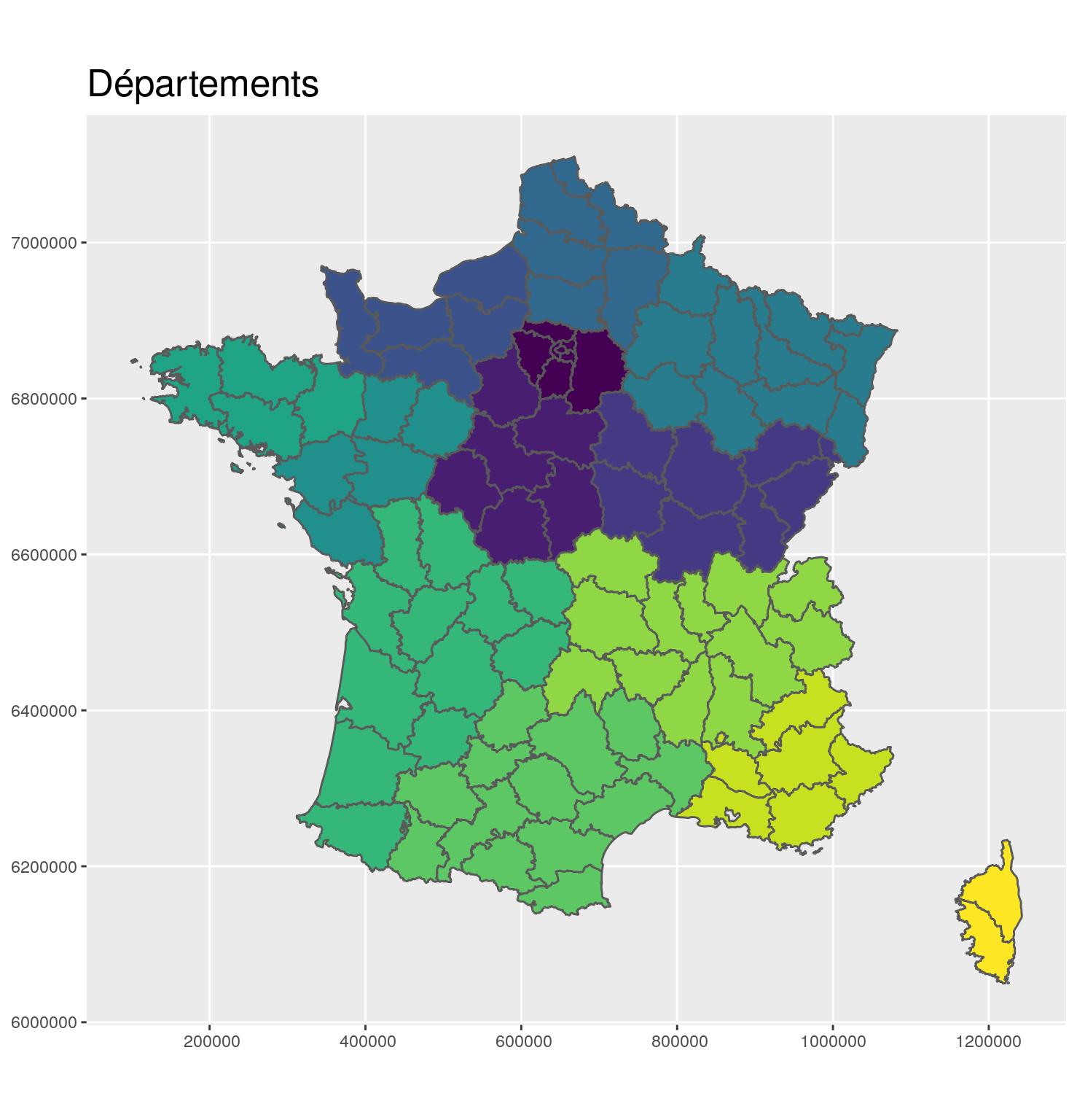
Merge
region_L93 <- departements_L93 %>%
group_by(CODE_REG, NOM_REG) %>%
summarize()After
g_region <- ggplot(region_L93) +
aes(fill = CODE_REG) +
scale_fill_viridis_d() +
geom_sf() +
coord_sf(crs = 2154, datum = sf::st_crs(2154)) +
guides(fill = FALSE) +
ggtitle("Régions") +
theme(title = element_text(size = 16))
g_region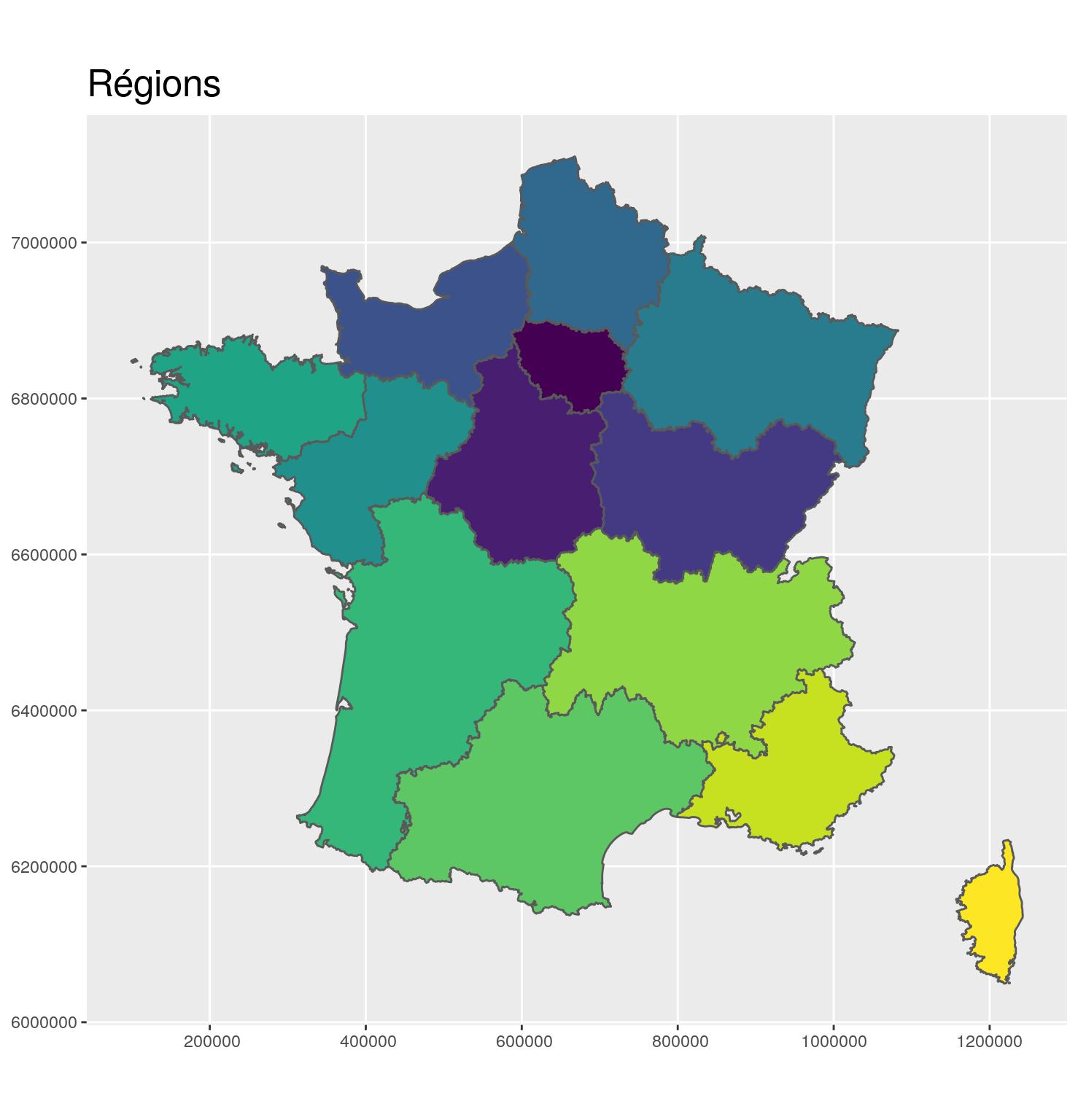
- Classical data join between a shapefile of French communes and a CSV file of French communes having a maternity with
left_join.- The map of communes comes from the ign website. You can download it on my github too.
- The maternity data come from the open-data portal of the French Ministry of Solidarity and Health. These are the “SAE - Annual Statistics on Health Facilities” databases. On my github here, a Rmd file describes how I prepared the maternity dataset.
Download the data
# extraWD <- "."
# -- Communes --
if (!file.exists(file.path(extraWD, "communes.zip"))) {
githubURL <- "https://github.com/statnmap/blog_tips/raw/master/2018-07-14-introduction-to-mapping-with-sf-and-co/data/communes.zip"
download.file(githubURL, file.path(extraWD, "communes.zip"))
}
unzip(file.path(extraWD, "communes.zip"), exdir = extraWD)
# -- Maternites --
if (!file.exists(file.path(extraWD, "communes.zip"))) {
githubURL <- "https://github.com/statnmap/blog_tips/raw/master/2018-07-14-introduction-to-mapping-with-sf-and-co/data-mater/Maternite_2004-2016.csv"
download.file(githubURL, file.path(extraWD, "Maternite_2004-2016.csv"))
}
# Read shapefile of French communes
communes <- st_read(dsn = extraWD, layer = 'COMMUNE', quiet = TRUE) %>%
select(NOM_COM, INSEE_COM)
# Read file of maternities for 2016
data.maternite <- readr::read_csv(file.path(extraWD, "Maternite_2004-2016.csv")) %>%
filter(an == 2016)Jointure
# Join database with shapefile by attributes
maternites_L93 <- communes %>%
right_join(data.maternite,
by = "INSEE_COM") %>%
st_transform(2154) g_region +
geom_sf(data = maternites_L93, fill = "white", colour = "white") +
coord_sf(crs = 2154, datum = sf::st_crs(2154)) +
ggtitle("Communes avec une maternité en 2016")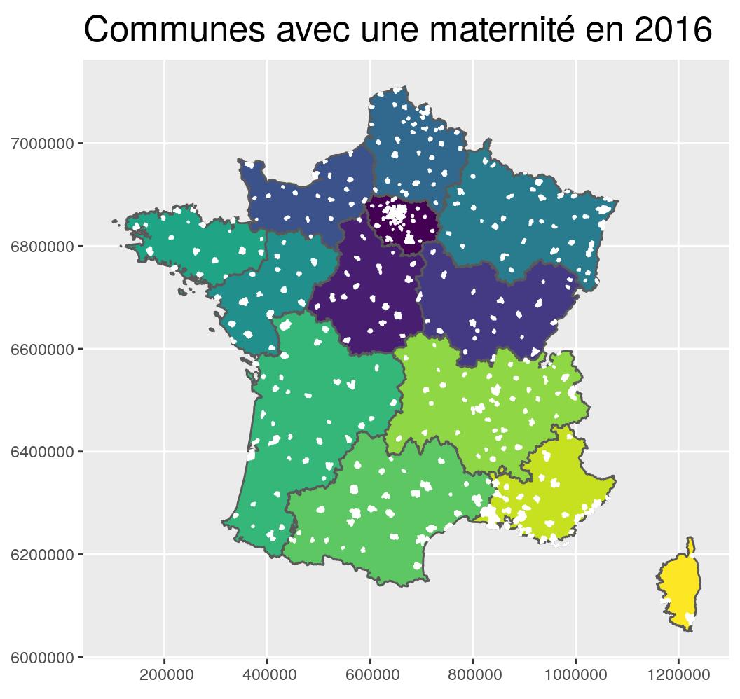
Spatial join
Join layers with st_intersection to spatially select and retrieve information from another spatial layer based on geographic positions.
- Points, polygons, lines with polygons
Spatial join
maternites_Bret_L93 <- maternites_L93 %>%
st_intersection(Bret_L93)## Attributs du fichier 'Maternités' avant intersection## [1] "NOM_COM" "INSEE_COM" "an" "Code_Postal" "n"
## [6] "geometry"## Attributs après Intersection avec région## [1] "NOM_COM" "INSEE_COM" "an" "Code_Postal" "n"
## [6] "CODE_DEPT" "NOM_DEPT" "NOM_REG" "geometry"ggplot() +
geom_sf(data = departements_L93, colour = "grey20") +
geom_sf(data = Bret_L93, fill = "#440154", colour = "grey60") +
geom_sf(data = maternites_Bret_L93,
fill = "#FDE725", colour = "#FDE725") +
coord_sf(crs = 2154, datum = sf::st_crs(2154),
xlim = st_bbox(Bret_L93)[c(1,3)],
ylim = st_bbox(Bret_L93)[c(2,4)]
) +
theme(title = element_text(size = 16),
panel.background = element_rect(fill = "#66BDFF")) +
ggtitle("Communes bretonnes avec maternité")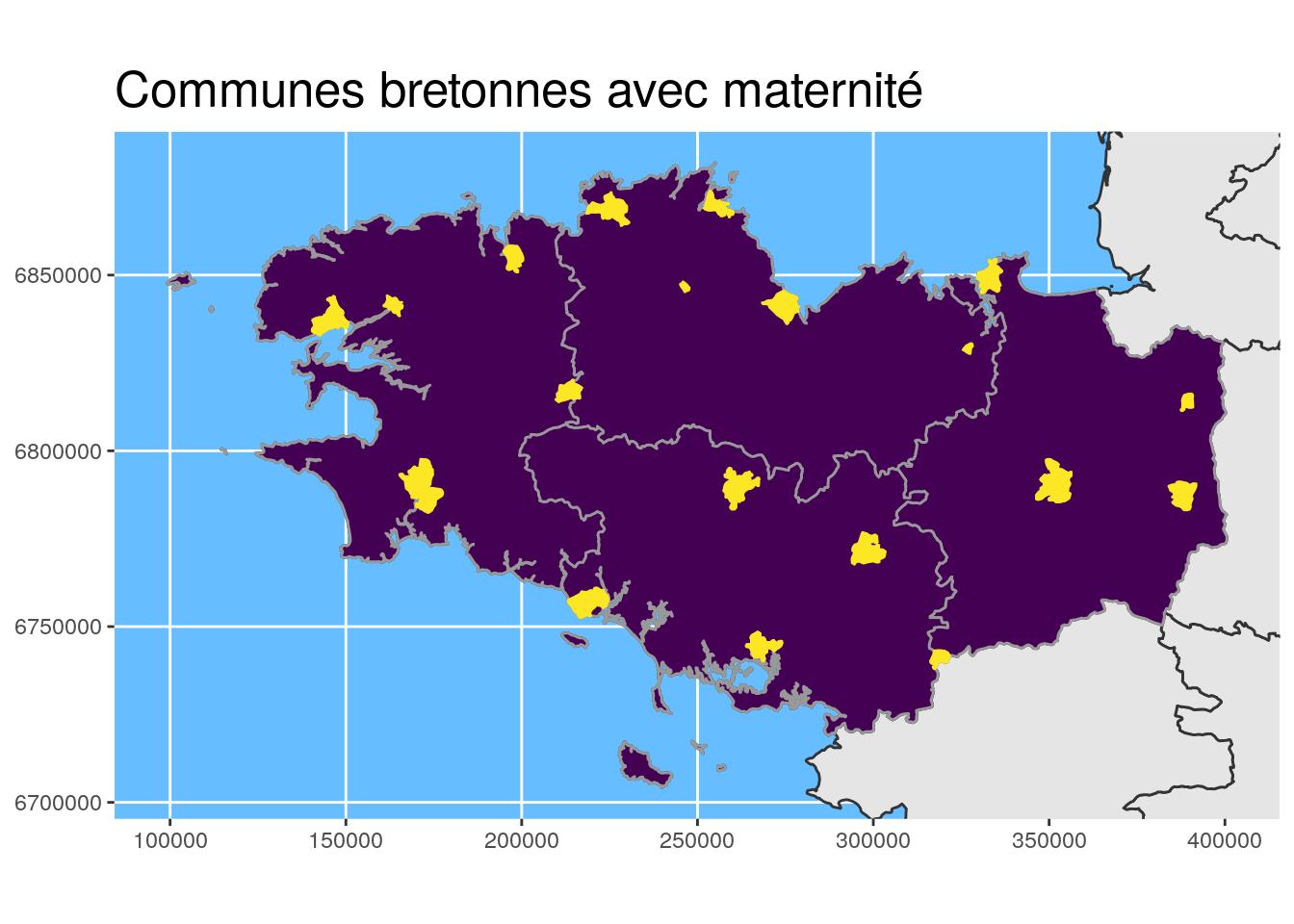
Geomatics
- Buffer area calculation to highlight the Brittany region with
st_buffer
Buffer area
# Buffer area for Brittany
Bret_buffer10_L93 <-
Bret_L93 %>%
st_buffer(
dist =
units::set_units(10, km)
) %>%
st_cast() # useful sometimes !
# Buffer Bretagne for larger study area bbox only
Bret_buffer30_L93 <-
Bret_L93 %>%
st_buffer(
dist =
units::set_units(30, km)
) ggplot() +
geom_sf(data = departements_L93, colour = "grey50",
fill = "white") +
geom_sf(data = st_union(Bret_buffer10_L93), fill = "#FDE725", #"#440154",
colour = "grey80", size = 1.1) +
geom_sf(data = st_union(departements_L93), colour = "grey20",
fill = NA, size = 1.2) +
geom_sf(data = Bret_L93, fill = "#440154", colour = "grey60") +
# scale_fill_manual(values = c("#f15522", "#15b7d6", "#ada9ae")) +
coord_sf(crs = 2154, datum = sf::st_crs(2154),
xlim = st_bbox(Bret_buffer30_L93)[c(1,3)],
ylim = st_bbox(Bret_buffer30_L93)[c(2,4)]
) +
theme(title = element_text(size = 16),
panel.background = element_rect(fill = "#66BDFF")) +
ggtitle("Zone tampon autour de la Bretagne")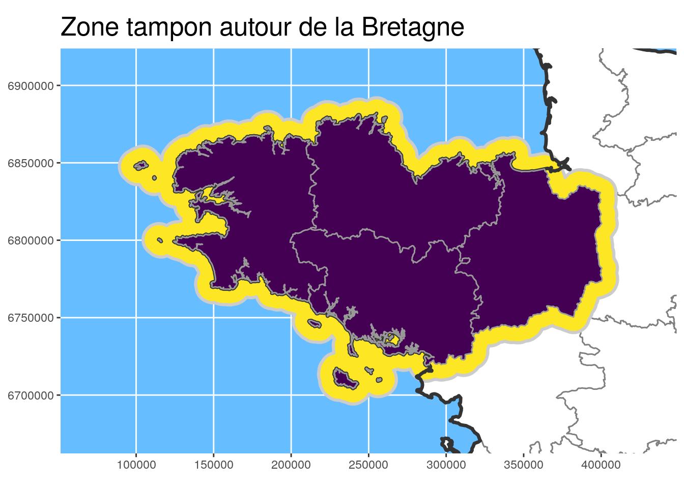
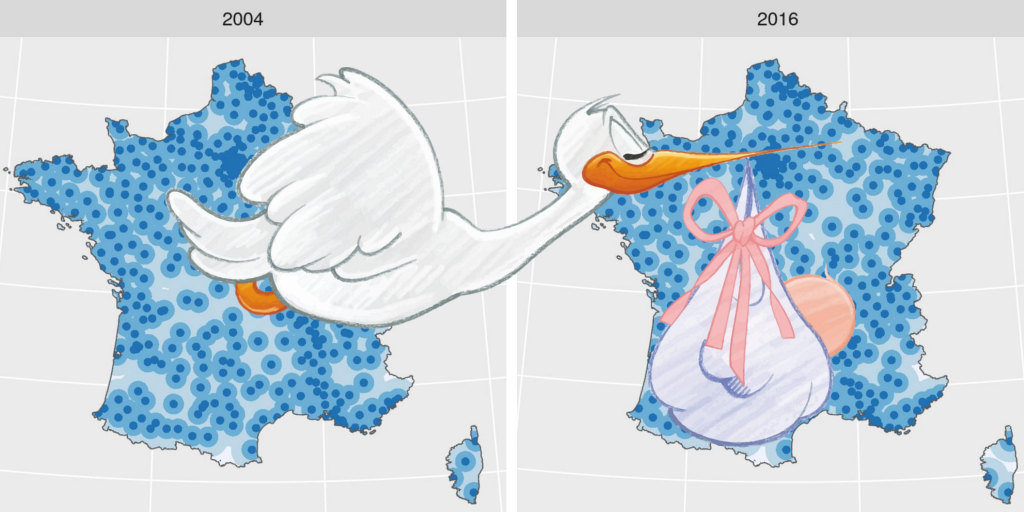
By coupling buffer areas with other utility functions, we can draw distance zones as the stork flies.
- Retrieve polygon centroids of communes in Brittany with a maternity with
st_centroid. - Unions with
st_union - Difference with
st_difference
In the code chunk below, the dist_circles function allows to create these buffer areas around a point or any other {sf} object.
Function
# Define couples distances - years to buffer
#' @param x sf object
#' @param dists c(10000, 25000, 50000, 75000)
#' @param ans unique(maternites_pt$an)
dist_circles <- function(x,
dists = units::set_units(c(10, 25, 50), km),
ans,
x.limits) {
# browser()
if (!missing(ans)) {
dists_ans <- data.frame(
dists = rep(dists, length(ans)),
ans = rep(ans, each = length(dists))
)
# Create buffer areas for each distances / year
pts_buf <- purrr::map2(
dists_ans$dists, dists_ans$ans,
~st_buffer(
filter(x, an == .y),
.x) %>%
mutate(
dist = .x,
)
) %>%
do.call("rbind", .) %>%
st_cast() %>%
mutate(dist.leg = glue::glue("<{dist/1000} km"))
# Define triplet big/small-distance/year
big_small <- data.frame(
big_dist = dists[rep(2:length(dists), length(ans))],
small_dist = dists[rep(1:(length(dists) - 1), length(ans))],
an = ans[rep(1:length(ans), each = length(dists) - 1)]
)
# Remove part of polygons overlapping smaller buffer
pts_holes <- big_small %>%
split(1:nrow(big_small)) %>%
purrr::map(
~st_difference(
filter(pts_buf, dist == .$big_dist, an == .$an),
filter(pts_buf, dist == .$small_dist, an == .$an)
)
) %>%
do.call("rbind", .) %>%
select(-contains(".1")) %>%
st_cast()
# Add smallest polygons and re-order distance names for legend
pts_holes_tot <- pts_holes %>%
rbind(
filter(pts_buf, dist == min(dists))
) %>%
arrange(an, dist) %>%
mutate(dist = forcats::fct_reorder(dist.leg, dist))
} else {
pts_buf <- purrr::map(
dists,
~st_buffer(x, .x) %>%
mutate(dist = .x)
) %>%
do.call("rbind", .) %>%
st_cast() %>%
mutate(dist.leg = as.character(dist))
# Define triplet big/small-distance/year
dists_order_char <- sort(dists) %>% as.character()
big_small <- data.frame(
big_dist = tail(dists_order_char, -1),
small_dist = head(dists_order_char, -1)
)
# Remove part of polygons overlapping smaller buffer
pts_holes <- big_small %>%
split(1:nrow(big_small)) %>%
purrr::map(
~st_difference(
filter(pts_buf, dist.leg == .$big_dist),
filter(pts_buf, dist.leg == .$small_dist) %>%
select(geometry) %>% st_union()
)
) %>%
do.call("rbind", .) %>%
select(-contains(".1")) %>%
st_cast()
# Add smallest polygons and re-order distance names for legend
pts_holes_tot <- pts_holes %>%
rbind(
filter(pts_buf, dist.leg == dists_order_char[1])
) %>%
arrange(dist) %>%
mutate(dist = forcats::fct_reorder(dist.leg, dist))
}
pts_holes_fr <- st_intersection(pts_holes_tot,
dplyr::select(x.limits, geometry))
return(pts_holes_fr)
}Calculation of distance circles
# Centroides des communes des maternités
maternites_centroid_Bret_L93 <-
maternites_Bret_L93 %>%
st_centroid()
# Circles around centroids
dists <- c(5, 15, 25, 50)
maternites_circles_L93 <- dist_circles(
maternites_centroid_Bret_L93,
dists = units::set_units(dists, km),
x.limits = Bret_L93)Figure
# Plot and define color according to dist
ggplot() +
geom_sf(data = departements_L93, colour = "grey50",
fill = "white") +
geom_sf(data = st_union(Bret_buffer10_L93), fill = "#FDE725", #"#440154",
colour = "grey80", size = 1.1) +
geom_sf(data = maternites_circles_L93,
aes(fill = dist),
colour = NA) +
scale_fill_brewer(direction = -1) +
geom_sf(data = Bret_L93, fill = NA, colour = "grey60") +
geom_sf(data = st_union(departements_L93), colour = "grey20",
fill = NA, size = 1.2) +
# scale_fill_manual(values = c("#f15522", "#15b7d6", "#ada9ae")) +
coord_sf(crs = 2154, datum = sf::st_crs(2154),
xlim = st_bbox(Bret_buffer30_L93)[c(1,3)],
ylim = st_bbox(Bret_buffer30_L93)[c(2,4)]
) +
theme(title = element_text(size = 16),
panel.background = element_rect(fill = "#66BDFF")) +
ggtitle("Distances à vol d'oiseau du centre\nd'une commune avec maternité")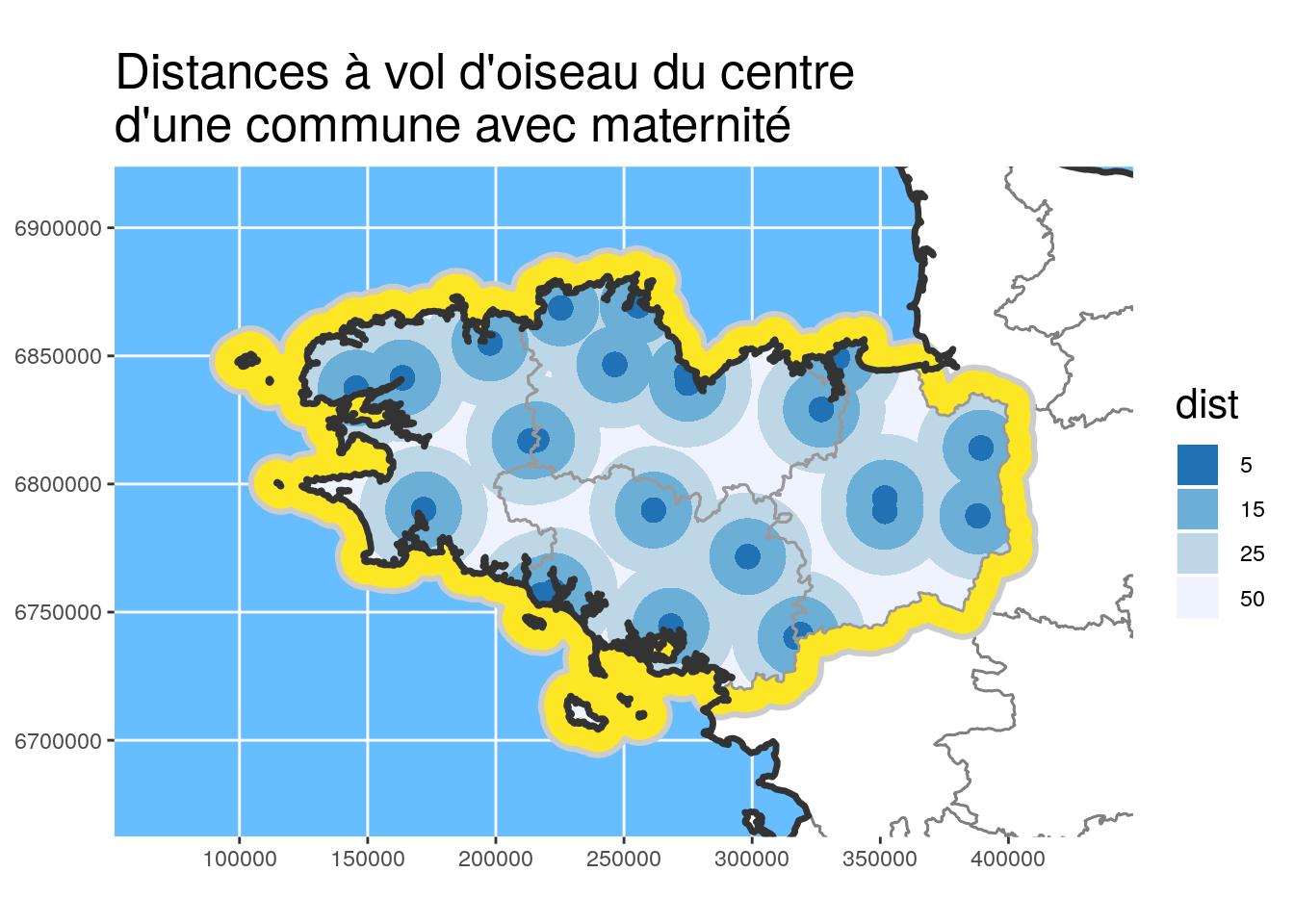
I used a similar technique in my previous article “Polygons tint bands with leaflet and package {sf}”
Draw maps on R
non-exhaustive personal list of the tools I use the most.
Maps with {ggplot2}
You may have noticed that the previous maps were all made with {ggplot2}. It is now possible with the last version of {ggplot2} (v3.0+) recently released on CRAN ! I also put {viridis} colours in the previous maps because it is also possible in a simple way with scale_fill_viridis_* in the new version of {ggplot2}. If you want to know more about {viridis}, have a look at Viridis ThinkR blog post.
geom_sf: recognizes geometrycoord_sf: axis limits and CRS- Several layers can be added by specifying
geom_sf(data = ...)
ggplot() +
geom_sf(data = departements_L93, colour = "grey40",
fill = "white", size = 1.1) +
geom_sf(data = maternites_circles_L93,
aes(fill = dist), colour = NA) +
scale_fill_brewer(direction = -1) +
coord_sf(crs = 2154, datum = sf::st_crs(2154),
xlim = st_bbox(Bret_buffer30_L93)[c(1,3)],
ylim = st_bbox(Bret_buffer30_L93)[c(2,4)]
) +
theme(title = element_text(size = 16),
panel.background = element_rect(fill = "#66BDFF")) +
ggtitle("Distances à vol d'oiseau du centre\nd'une commune avec maternité")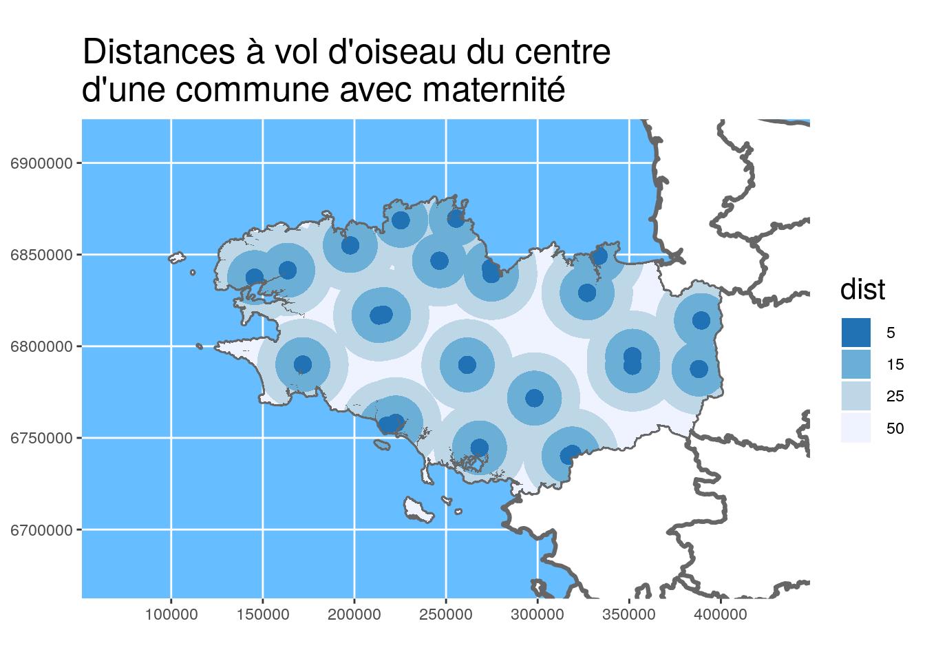
Maps with {tmap}
I like {tmap} because it was created to draw maps. Different spatial data formats are supported ({sp}, {sf}, {raster}), North scale and arrow are managed natively. You can add multiple layers on top of each other using tm_shape.
Some functions :
tm_shapetm_dots: pointstm_fill: polygonstm_text: text
tm_scale_bartm_compass
# Load background map
# data(Europe) # deprecated in tmap 2.0
data(World)
Europe <- World %>%
filter(continent == "Europe" & name != "France")
# Map
tm <- tm_shape(Europe) +
tm_polygons() +
tm_shape(departements_L93, is.master = TRUE) +
tm_fill(col = "NOM_DEPT", legend.show = FALSE, palette = "Set1") +
tm_borders("grey30") +
tm_shape(maternites_circles_L93) +
tm_fill(col = "dist", palette = "-Blues") +
tm_scale_bar(position = c("right", "bottom"), size = 1) +
tm_compass(position = c("right", "top"), size = 1.8) +
# tm_style_natural() #deprecated in tmap 2.0
tm_style("natural")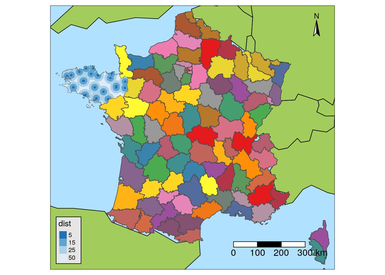
Interactive maps with {leaflet}
To provide interactive maps, you can use {leaflet}:
- Accept {sf} objects
- CRS: 4326
- Create color palettes with
colorFactorfor example addTiles(): Maps in backgroundaddMarkers: PointsaddPolygons: Polygons
departements_wgs84 <-
st_transform(departements_L93, crs = 4326)
factpal <- colorFactor(topo.colors(5), departements_wgs84$NOM_REG)
m <- leaflet() %>%
addTiles() %>%
addPolygons(data = departements_wgs84,
color = ~factpal(NOM_REG),
fillOpacity = 0.8, stroke = FALSE)
mInteractive maps with {leaflet} and {tmap}
The magic of {tmap} works here: with tmap_leaflet, you can transform your map {tmap} into an interactive map ! No need to learn the leaflet syntax, {tmap} does the magic trick for you!
tmap_leaflet(tm)Get rid of QGIS (or others)?
Until recently, there was no way to view and explore the space objects produced in R interactively at a glance. This time is over thanks to {mapview} and its mapView and viewRGB functions!
library(mapview)
mapView(departements_L93)Even better, by coupling {mapview} with {mapedit}, it is now possible to create and digitalize spatial objects directly and interactively with the editMap function! Could we now work without traditional mapping software such as QGIS? Time will tell… Anyway,this is very interesting, for instance, to integrate interactive mapping into Shiny Apps!
As an example, I used these packages in the blog article for ThinkR: The ThinkR logo created with the {sf}.
logo_pol <- viewRGB(logo) %>% editMap()
logo_overlap <- logo_pol$finished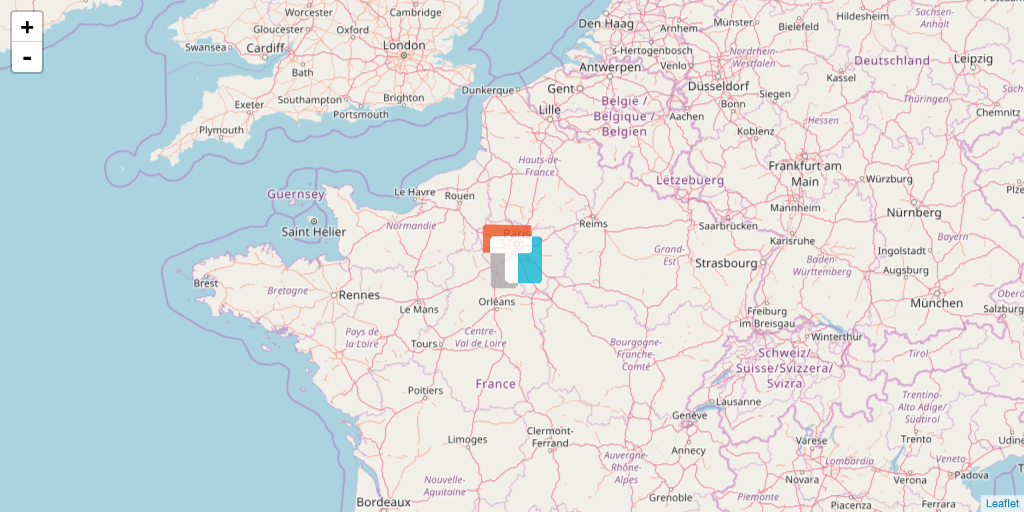
There you go. It’s over for this presentation of tools I regularly use to do mapping in R. The functions proposed by {sf} are much more numerous than the few I presented here. And of course, there are other ways to draw maps in R. You could look at the packages {cartography}, {ggmap} or the recent {ggspatial} for example.
The future of mapping in R is bight !
Now that you know how to create maps with R, you can read these specific articles:
- Create maps in R with {ggplot2}
- Create maps in R with {tmap}
- Create maps with a spherical view at the globe scale
The complete R script of this article and all data used can be found on my Blog Tips Github repository.
Citation:
For attribution, please cite this work as:
Rochette Sébastien. (2018, Jul. 14). "Introduction to mapping with {sf} & Co.". Retrieved from https://statnmap.com/2018-07-14-introduction-to-mapping-with-sf-and-co/.
BibTex citation:
@misc{Roche2018Intro,
author = {Rochette Sébastien},
title = {Introduction to mapping with {sf} & Co.},
url = {https://statnmap.com/2018-07-14-introduction-to-mapping-with-sf-and-co/},
year = {2018}
}